The basic model of queueing theory
The queuing theory uses a simple basic model to describe operation of systems. It consists of the so-called service station which has one or more parallel operating similar machines or operators, and a waiting room. The clients arrive at individual random times at the service station. A newly arrived customer is served, if at least one of the operating units is available, otherwise ha has to wait in the queue.

The basic model can be varied in many ways:
- Customers are not served individually, but in groups (waiting systems with batch operation). Application: producing batches in a production plant
- Some customers leave the system before they are served (waiting systems with time restrictions). Application: storage of perishable goods
- Not all service devices are available for all customer (service systems with limited accessibility). Application: production lines with dedicated machines, switching arrangements in a telephone network.
- Some customers reject to enter the queueing system, because they the queue appears to too long for them (queueing systems with impatient customers). Application: common customer behavior at a post office, bank or ticket office
- A customer with a higher priority displaces customers lower priority from the service process (service systems with priority control). Application: Express lanes in a manufacturing process
- A customer who can not be served immediately upon his arrival, is lost (loss systems). Application: telephone calls in a telephone network
The flow of incoming requests is described by a so-called renewal process. For this purpose we imagine all requests are numbered in the in the order of their arrival. The time span In between the arrival of the (n-1)-th and the n-th customer is called inter-arrival time. The random variables In, n = 1, 2, ..., are assumed to be distributed stochastically independent and identical with the distribution function Fl(x), the expected value E[I] and the variance D[I]. The reciprocal

is called the arrival rate and indicates how many customers will arrive at the system come in average per time unit.
The service times Sn, n = 1, 2, ..., of the successive customers also interpreted as stochastically independent and identically distribute random variables. The distribution function of the service times is denoted by FS(x). For the corresponding expected value and the associated variance we use the symbols E[S] and D[S]. The reciprocal

is called service rate and indicates how many customers can be handled by the operation system per time unit in average. If there are several parallel and similar operation equipment available, the operating rate increased according to the number of devices.
The operation policy determines the order in which waiting customers are handled. The following rules and terms are used:
| FIFO (FCFS) | First In, First Out (First Come, First Served). The clients are served in the order of arrivals. | |
| LIFO (LCFS) | Last In, First Out (Last Come, First Served). The clients are served in the reverse order of arrivals. | |
| SIRO | Selection In Random Order. The next client is chosen at random. | |
| Non-preemptive priority | Relative priority. Some clients will be served with a higher priority. The operation of a client already in process will be continued before serving a client with an higher priority. | |
| Preemptive priority | Absolute priority. If a newly arrived customer has a higher priority than the client which is just in operation, the service process will be stopped, so the client with the higher priority can be served immediately. | |
| RR | Round Robin. Each client can use the service station for a certain period of time. Clients whose handling requires more time, therefore have to enter the queue multiple times. |
For symbolic markup of operating systems D.G. Kendall and B. W. Gnedenko have introduced the notation
A / B / c /m
The letters A and B here define the distribution type of the inter-arrival times and the service times. The letter c represents the number of parallel servers and m refers to the capacity of the waiting room.
The following abbreviations are used for the distribution type:
| D | Deterministic distribution |
| M | Exponential distribution |
| Ek | Erlang distribution with parameter k (k = 1, 2, ...) |
| Hk | Hyper-exponential distribution with parameter k (k = 1, 2, ...) |
| PH | Phase-type distribution |
| G | General distribution |
Example: The notation M/G/3/5 denotes an queueing system with exponentially distributed inter-arrival times, randomly distributed service times, three parallel servers and a waiting room, where a maximum 5 clients can wait.
The performance evaluation of queueing systems is based on the following processes:
- The number of clients in the system (Nt)t>0. This process describes how many clients are in the system at the time t.
- The process of successive staying times (or lead times) (Vn)n in N. The random variable Vn describes the time the n-te client will stay in the system.
For computations of the basic parameters different methods of the theory of stochastic processes can be used. The suitability of a method depends on what types of distributions are used for the inter-arrival and the service times and whether time-dependent or stationary values are to be calculated. Even the basic model of queueing theory is so complicated that it can not be solved exactly under general distribution assumptions. However, there are approximate formulas, which have proven themselves quite well in practice and make the stochastic operation of service systems transparent. By the formula of Allen-Cunnen the average number of customers in the stationary case is:

Here ρ means the utilization of the systems, root(ρc+1) the waiting probability and cI2 and cS2 the coefficients of variation of the inter-arrival and service times. The formula tells us that the number of clients in the system is larger if the load on the system and the coefficients of variation are larger. To get a small queues, therefore you have to provide sufficient capacity or keep the variability of the system low.
The average staying time time is obtained using the formula of Little:

where λ describes the input rate at the system.
The formulas can be used to illustrate the following relationships:

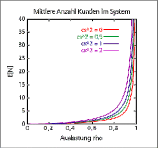
The average number of customers in the system depends on the utilization of the operating station. If the utilization ρ is increasing, the number of clients in the system will grow, too. One can also observe: The larger the coefficient of variation of the operating time is, the larger is also the average number of customers in the system E[N].

The average staying time E[V] is obviously correlated with the average number of customers in the system. The larger the utilization and the variability of the system, the longer the clients will have to wait.

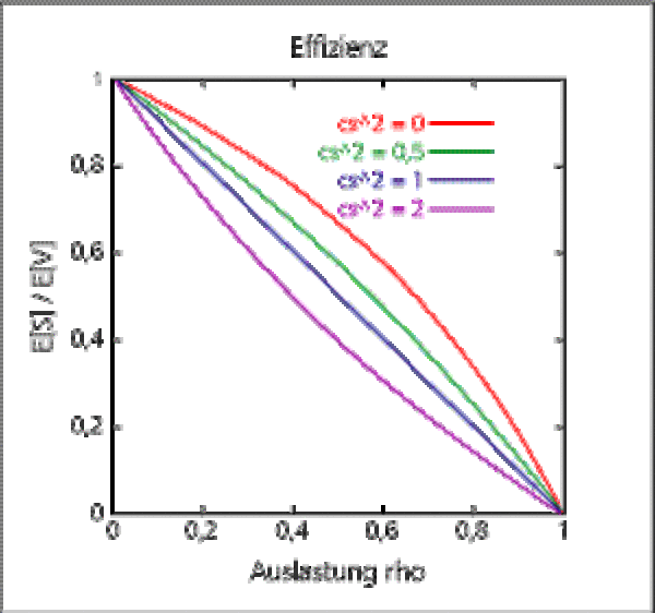
The ratio of pure service time to the total staying time of a client is called his efficiency. Since the stying time increases to any number with increasing utilization, the efficiency is aiming towards zero.

Our formula also allows to describe the utilization level ρdepending on the WIP (work units in process) E[N]. The graph shows that one achieves not higher throughput at a certain load factor, despite higher stocks. That's for example why new orders in production processes should not be added before the stock falls below a critical level (so-called load-oriented order release).


